This page contains extra R content not covered in the demonstrations and could be considered supplementary to the module. This content is useful for completing the advanced exercises from Week 6 and focuses on conducting logistic regression in R. Logistic regression is typically used when the DV is categorical with one or more continuous IV.

Logistic Regression

A logistic regression is used when you have a categorical DV and a continuous IV. The most simple scenario is when the DV is binary (i.e., only has two categories). The two categories of the DV coded as 0 and 1.

To conduct a logistic regression in R, you can use the glm() function. In this instance, ‘glm’ stands for Generalised Linear Model, and can be used for many different types of analysis. Like most analysis functions, the glm() function accepts a formula and a data.frame. We also need to tell the function which type of analysis to conduct. This is done via the family argument. To conduct a binomial logistic regression, we set this argument to “binomial”. Much like with the lm() function, to view the results in an interpretable way you must use the summary() function.

Altogether, this becomes:

#The DV must be a categorical variable with two levels.
model <- glm(DV ~ IV,data = data,family = "binomial")
summary(model)

1. Prepare Data for Analysis

Let’s look an example using the class data. Let’s say that you predict that people who are more introverted are more likely to play videogames than not. A logistic regression is appropriate because you have a continuous IV (introversion score) and a categorical DV (videogamer vs. non-videogamer). Importantly, the two groups for the outcome variable must be coded as 0 and 1. We can use the ifelse() function inside a mutate() function to achieve this. You can also do this by changing the variable class to a factor.

First, let’s prepare the data by calculating the necessary scores. We have also loaded the necessary packages, being tidyverse.

library(tidyverse)

analysis.data <- data %>%
  mutate( introvert = introversion2 + introversion5 + introversion7 + introversion8 + introversion10,
          video.games = ifelse(video.games == "Yes",1,0)) %>%
  select(introvert,video.games)

2. Conduct the Statistical Test

Following the example above, we can use the glm() function to conduct the logistic regression.

model <- glm(video.games ~ introvert,data = analysis.data,family = "binomial")

summary(model)

## 
## Call:
## glm(formula = video.games ~ introvert, family = "binomial", data = analysis.data)
## 
## Coefficients:
##             Estimate Std. Error z value Pr(>|z|)  
## (Intercept)  2.33519    0.97050   2.406   0.0161 *
## introvert   -0.14552    0.07028  -2.071   0.0384 *
## ---
## Signif. codes:  0 '***' 0.001 '**' 0.01 '*' 0.05 '.' 0.1 ' ' 1
## 
## (Dispersion parameter for binomial family taken to be 1)
## 
##     Null deviance: 107.68  on 79  degrees of freedom
## Residual deviance: 103.03  on 78  degrees of freedom
## AIC: 107.03
## 
## Number of Fisher Scoring iterations: 4

3. Write-up the Results

Much like with a standard regression, you get statistics about overall model performance, as well as statistics for each individual predictor. Similarly, you are expected to report both for a logistic regression. For the statistics for each predictor, however, there is not one standard way to report a logistic regression. Some people choose to report the unstandardised coefficients, z-statistic, and associated p-values as given in the summary() function. Others choose to convert these to odds-ratios and report 95% confidence intervals. You can use the following code if you want to convert the coefficients to odds-ratios.

exp(cbind(OR = coef(model), confint(model)))

##                     OR     2.5 %     97.5 %
## (Intercept) 10.3314267 1.6768661 78.3328287
## introvert    0.8645688 0.7472052  0.9871924

4. Visualise the Data

To visualise a logistic regression, we can plot the probabilities. To do this, we can use the geom_jitter() and geom_smooth() functions, similar to with a standard regression.

How to read the graph below is the line represents the probability of being in one of the two groups (0 = non-videogamers, 1 = videogamers) for each level of the variable on the x-axis (introversion). If there is a strong relationship, then the logistic regression line should have a very characteristic “S” shape. If there is no relationship, the logistic regression line will look quite straight. Note that since participants can only be in one of two groups, all the points will either be at the top, or bottom of the y-axis.

There are a few things to note: 1), I have adjusted the height, width and alpha aesthetics in the geom_jitter() function so it makes it a bit easier to see all the individual points; and 2) we need to adjust the method and method.arg arguments in the geom_smooth() function to create a logistic regression line.

ggplot(analysis.data,aes(x = introvert,y = video.games)) +
  geom_jitter(height = .05,width = 0,alpha = .3) +
  geom_smooth(method = "glm",method.args = list(family = "binomial"),se = FALSE) +
  theme_classic()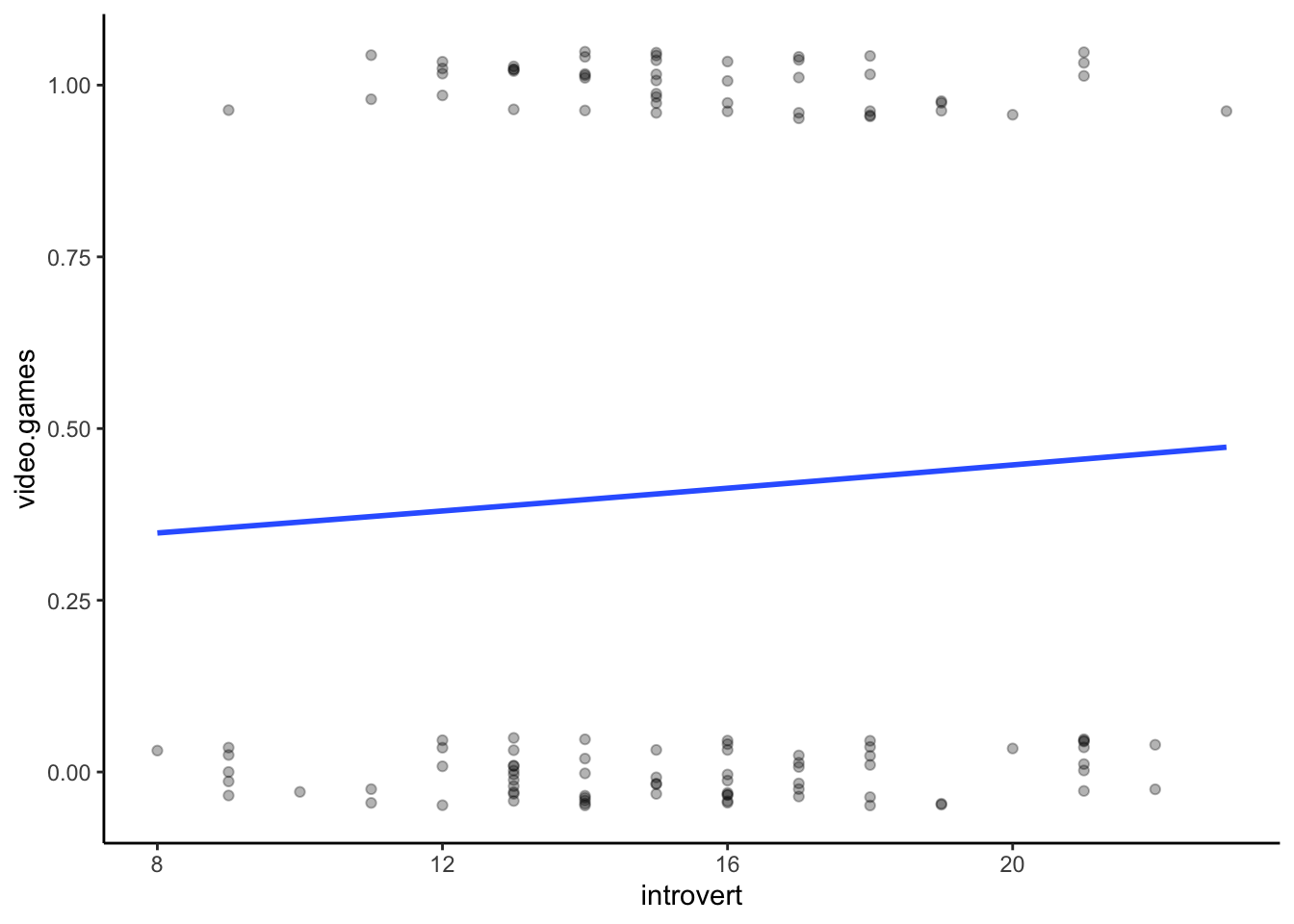

Advanced Exercises

If you would like to practice the skills on this page, weekly exercise questions on this content are available in the advanced exercises for Week 6. You can download the interactive exercises by clicking the link below.

Click here to download this week’s exercises.