Content

These are the packages we will be using in this workbook. If you’ve been following the workbook sequentially, you should be familiar with the tidyverse and lm.beta packages. The pwr package is used to conduct standard power analyses, while the psych package has many useful functions; however, we will just be using it to run a mediation analysis via bootstrapping.

library(pwr)
library(tidyverse)
library(lm.beta)

pwr Package

For most standard analyses, such as an independent-samples t-test, the easiest way to conduct power analyses is by using functions in the pwr package. Functions from the pwr package work by specifying three of four bits of information that influence statistical power: the expected effect size, power threshold, and significance level (alpha), and the sample size. The function will then return whichever of the four parts was not specified. Typically, power analyses are used to calculate the sample size required before a study is conducted; therefore, this is what we will be focusing on here.

We will cover four examples: a power analysis for a correlation, an independent-samples t-test, a one-way ANOVA, and a multiple regression.

pwr and correlations

To conduct a power analysis for a correlation, we can use the pwr.r.test() function. This function expects three of four arguments:

n = Sample Size
r = Expected Effect size
sig.level = Significance Level
power = Power threshold

As discussed in the lecture, things like the significance level and power threshold are already chosen for you. Conventionally, the significance level is set to .05, while the power threshold is .80 (80%). Therefore, you only need to decide the expected effect size to calculate the required sample size.

Recall from the lecture series the following interpretation:

Effect size	r
Small	.10
Medium	.30
Large	.50

Therefore, if we needed to calculate the required sample size for a correlation where you expect a medium effect, you could use the following code:

pwr.r.test(r = .30,sig.level = .05,power = .80)

## 
##      approximate correlation power calculation (arctangh transformation) 
## 
##               n = 84.07364
##               r = 0.3
##       sig.level = 0.05
##           power = 0.8
##     alternative = two.sided

This would indicate that we would require a sample of 85 participants (rounded-up) to detect a medium effect. By playing around with the expected effect size, we can see how this impacts the required number of participants. For instance, if we expect a small effect, we will need a much larger sample size:

pwr.r.test(r = .10,sig.level = .05,power = .80)

## 
##      approximate correlation power calculation (arctangh transformation) 
## 
##               n = 781.7516
##               r = 0.1
##       sig.level = 0.05
##           power = 0.8
##     alternative = two.sided

pwr and t.tests

Similarly, we can use pwr.t.test() to conduct a power analysis for an independent-samples t-test. However, one thing to note is that the expected effect size for this function is a Cohen’s d. Therefore, we can use the following conventions:

Effect size	d
Small	.20
Medium	.50
Large	.80

So, if we expect a medium effect, the code would be:

pwr.t.test(d = .50,sig.level = .05,power = .80)

## 
##      Two-sample t test power calculation 
## 
##               n = 63.76561
##               d = 0.5
##       sig.level = 0.05
##           power = 0.8
##     alternative = two.sided
## 
## NOTE: n is number in *each* group

Note that the expected effect size is the minimum for each group. Therefore, you would need a total sample of 128 participants (rounded-up).

pwr and ANOVAs

For a one-way ANOVA, we can use the pwr.anova.test() function. This analysis assumes there will be equal numbers in each group. Again, this function uses another measure of effect size, Cohen’s f, which you can use the following interpretations:

Effect size	f
Small	.10
Medium	.25
Large	.40

This function also requires an additional parameter k, which is the number of levels (or groups) in the IV. So, if you were conducting a one-way ANOVA with three groups in the IV, and expect a medium effect, the code would look like this:

pwr.anova.test(k = 3,f = .25,sig.level = .05,power = .80)

## 
##      Balanced one-way analysis of variance power calculation 
## 
##               k = 3
##               n = 52.3966
##               f = 0.25
##       sig.level = 0.05
##           power = 0.8
## 
## NOTE: n is number in each group

Again, the value provided for n is for each group, so you would need a total of 159 participants (rounded-up).

pwr and multiple regressions

For a power analysis for a multiple regression, we use pwr.f2.test(). Annoyingly, we again have a different measure used for effect size again - f2. You can follow this guide to get your estimated effect size (I’ve also added a column with the corresponding R-square value):

Effect size	f2	R-square
Small	.02	.02
Medium	.15	.13
Large	.35	.26

For the pwr.f2.test() function, you need to also specify the number of predictors in the model as the argument u. Note, if you have an interaction term in your analysis, this counts as an additional predictor. As an example, if you were conducting a multiple regression with 4 predictors and expect a medium effect, the code for the power analysis would look like:

pwr.f2.test(u = 4,f2 = .15,sig.level = .05,power = .80)

## 
##      Multiple regression power calculation 
## 
##               u = 4
##               v = 79.44992
##              f2 = 0.15
##       sig.level = 0.05
##           power = 0.8

Therefore, you would need at least 80 participants for this study. Note that the power analysis in this instance is for the overall model (i.e., for the variance in the outcome variable that is explained by all the predictors in the regression).

Power Analyses via Simulations.

Above, we cover functions that allow you to conduct power analyses for common statistical techniques used in psychological research. However, if you are dealing with a more complicated design/statistical test, then these easy-to-use functions become less helpful. One way to conduct a power analysis is via simulation. For more information on this, see this extra content page.

Mediation

As covered in the lecture series, mediation describes a relationship where the influence of one variable on another can be explained through a third variable. In the example below, we will test whether the relationship between attitudes towards exercise and exercise behaviour can be explained through intentions to exercise (i.e., individuals who have positive attitudes about exercise increase their intention to exercise, which in turn increases exercise behaviour). For more information on these scales (and some of the ones we will use later), see this paper: https://search.proquest.com/docview/202682863. Note, we only use the first 5-items on each scale to keep things simple.

1. Clean data for analysis.

First, we must calculate the variables that we need for our analysis. This process should be fairly familiar by now. Note: due to a coding error, there is one participant that needs to be removed for having scores outside the possible range (not sure how that happened!). That is what the last line of this code chunk is doing.

data.clean <- data %>%
  mutate(attitude = exercise.attitude.1 + exercise.attitude.2 + exercise.attitude.3 + exercise.attitude.4 + exercise.attitude.5,
         intention = exercise.intention.1 + exercise.intention.2 + exercise.intention.3 + exercise.intention.4 + exercise.intention.5,
         behaviour = exercise.behaviour.1 + exercise.behaviour.2 + exercise.behaviour.3 + exercise.behaviour.4 + exercise.behaviour.5) %>%
  dplyr::select(student.no,attitude,intention,behaviour) %>%
  filter(!is.na(attitude)) %>%
  filter(!is.na(intention)) %>%
  filter(!is.na(behaviour)) %>%
  filter(intention <= 15)

2. Run statistical test

Remember, mediation is when the effect of one IV could be explained through a third variable (mediation). If there is an effect in a model without the mediator, but that effect is reduced (or disappears) when the mediator is included, there is a chance the mediation is happening. In order to check whether our variables meet these conditions, we need to conduct a series of linear regressions.

Model 1

Here, we test whether there is an association between the predictor (attitudes) and the outcome variable (behaviour):

lm(behaviour ~ attitude,data = data.clean) %>%
  lm.beta() %>%
  summary()

## 
## Call:
## lm(formula = behaviour ~ attitude, data = data.clean)
## 
## Residuals:
##      Min       1Q   Median       3Q      Max 
## -11.5297  -2.9735   0.2323   3.2323  11.4091 
## 
## Coefficients:
##             Estimate Standardized Std. Error t value Pr(>|t|)    
## (Intercept) 15.94456           NA    0.40818  39.063   <2e-16 ***
## attitude     0.17685      0.17285    0.09277   1.906    0.059 .  
## ---
## Signif. codes:  0 '***' 0.001 '**' 0.01 '*' 0.05 '.' 0.1 ' ' 1
## 
## Residual standard error: 4.47 on 118 degrees of freedom
## Multiple R-squared:  0.02988,    Adjusted R-squared:  0.02166 
## F-statistic: 3.634 on 1 and 118 DF,  p-value: 0.05904

Model 2

Here, we test whether including the mediator (intention) in the model changes the relationship between the predictor (attitude) and the outcome variable (behaviour):

lm(behaviour ~ attitude + intention,data = data.clean) %>%
  lm.beta() %>%
  summary()

## 
## Call:
## lm(formula = behaviour ~ attitude + intention, data = data.clean)
## 
## Residuals:
##      Min       1Q   Median       3Q      Max 
## -10.9129  -2.9535   0.1993   3.3387  11.3755 
## 
## Coefficients:
##             Estimate Standardized Std. Error t value Pr(>|t|)    
## (Intercept) 15.96246           NA    0.40986  38.946   <2e-16 ***
## attitude     0.16898      0.16516    0.09365   1.804   0.0737 .  
## intention   -0.06343     -0.06407    0.09061  -0.700   0.4853    
## ---
## Signif. codes:  0 '***' 0.001 '**' 0.01 '*' 0.05 '.' 0.1 ' ' 1
## 
## Residual standard error: 4.479 on 117 degrees of freedom
## Multiple R-squared:  0.03392,    Adjusted R-squared:  0.01741 
## F-statistic: 2.054 on 2 and 117 DF,  p-value: 0.1328

Model 3

Also, in order for there to be a mediation, we must observe a relationship between the predictor (attitude) and the mediator (intention):

lm(intention ~ attitude,data = data.clean) %>%
  lm.beta() %>%
  summary()

## 
## Call:
## lm(formula = intention ~ attitude, data = data.clean)
## 
## Residuals:
##      Min       1Q   Median       3Q      Max 
## -12.7859  -2.8169   0.1632   2.3748  12.3382 
## 
## Coefficients:
##             Estimate Standardized Std. Error t value Pr(>|t|)
## (Intercept)  0.28218           NA    0.41560   0.679    0.498
## attitude    -0.12408     -0.12005    0.09446  -1.314    0.192
## 
## Residual standard error: 4.551 on 118 degrees of freedom
## Multiple R-squared:  0.01441,    Adjusted R-squared:  0.00606 
## F-statistic: 1.725 on 1 and 118 DF,  p-value: 0.1915

Mediation Analysis

While we may or may not meet the conditions for a mediation above, we will continue with the analysis to demonstrate the process of conducting a mediation analysis regardless.

In order to conduct a mediation analysis in R, we will load the psych package. If you haven’t installed the psych package yet, make sure to do this before loading the psych package.

library(psych)

The function that runs the mediation analysis is aptly named mediate(). Like all analysis functions, the mediate() function accepts a formula and a data.frame, but also a couple of options that we will want to change. For the formula, the mediate function takes a specific form, where the mediator is put inside brackets on the right-hand side of the ~ symbol:

DV ~ IV + (Mediator)

So for our analysis, the code becomes the following. Note, we also want to set the ‘std’ argument to TRUE to ensure we receive standardised estimates, and the ‘plot’ argument to FALSE so we are only seeing the numeric output (we will see the plot later).

model <- mediate(behaviour ~ attitude + (intention),data = data.clean,std = TRUE,plot = FALSE)

model

## 
## Mediation/Moderation Analysis 
## Call: mediate(y = behaviour ~ attitude + (intention), data = data.clean, 
##     std = TRUE, plot = FALSE)
## 
## The DV (Y) was  behaviour . The IV (X) was  attitude . The mediating variable(s) =  intention .
## 
## Total effect(c) of  attitude  on  behaviour  =  0.17   S.E. =  0.09  t  =  1.91  df=  118   with p =  0.059
## Direct effect (c') of  attitude  on  behaviour  removing  intention  =  0.17   S.E. =  0.09  t  =  1.8  df=  117   with p =  0.074
## Indirect effect (ab) of  attitude  on  behaviour  through  intention   =  0.01 
## Mean bootstrapped indirect effect =  0.01  with standard error =  0.02  Lower CI =  -0.02    Upper CI =  0.05
## R = 0.18 R2 = 0.03   F = 2.05 on 2 and 117 DF   p-value:  0.11 
## 
##  To see the longer output, specify short = FALSE in the print statement or ask for the summary

Most of the information above is what we have encountered previously (e.g., we are given the total and direct effects that could be interpretted from the regressions above). The main information we are interested in this output is the line on the mean bootstrapped indirect effect. A large indirect effect (and consequently a greater drop between the total effect and the direct effect) would indicate that mediation is occurring. Since we are bootstrapping, we can tell the significance through confidence intervals. If the range between the lower CI and the upper CI contains zero, then the indirect effect is not significant (i.e., a population where the indirect effect is 0 could have produced our data). If this range does not contain zero, then we have a significant mediation effect.

3. Plot data

Path Diagram

For mediation, there’s no good way to plot the raw data that visualises the mediation. The most common way to visualise a mediated effect is through a path diagram. You can do this directly in the mediate() function by setting the ‘plot’ argument to TRUE or use the mediate.diagram() like below:

mediate.diagram(model)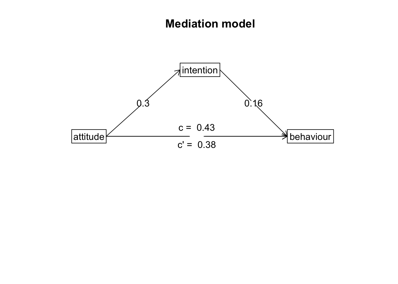

4. Write-up analysis.

There are several things you need to include when writing up a mediation analysis. Writing up a mediation analysis includes the write-up for each individual models with and without the mediator (Model 1 and Model 2 above - these numbers are also included in the output for the mediate() function), and also the estimated indirect effect and associated confidence intervals. Usually, you would want to accompany the write-up with a path diagram such as the one above. It does not make much sense to write-up the analysis above as we failed to meet the criteria for a mediation in the first instance, but if we were to do it anyway, it may go something like this:

In the model where attitudes towards exercise predicted variance in exercise behaviour, the effect of exercise attitudes was not significant (beta = 0.17, p = 0.059). When including intention to exercise into the model, the effect of attitudes on behaviour did not change (beta = 0.17, p = 0.074). Mediation analysis revealled a non-significant indirect effect of intentions to exercise on the association between attitudes towards exercise and exercise behaviour (mean bootstrapped indirect effect = 0.17, 95% CI = -0.02, 0.05).

Note: While we report the results in text above, it is sometimes also easier to report the separate models in a table.

HPSP131 - Workbook 8 - Power and Mediation

Objectives

Class Data

Exercises