Content

R

R is a programming language and free software environment for statistical computing and graphics. R is widely used by statisticians and data scientists. The use of R in psychological research has shown a substantial increase in popularity recently, given R’s superior ability to conduct advance statistical techniques, high level of community support, and ability to promote reproducible research. “Base R” consists of a “Read Evaluate Print Loop” (REPL) command interpreter, in which you type in text commands, which are evaluated, and the results of which are printed to the screen. Where you type in your commands for R to evaluate it is called the console.

RStudio

“Base R” can be unwieldy and lacks some quality-of-life features that makes using R difficult. In particular, when you are developing a script, you will want to work in a text editor and send commands to the console, rather than typing directly into the console. Thankfully, RStudio, which is a wrapper for Base R, provides this additional functionality and a graphical user interface that can make programming in R much easier. All teaching for this module will be done using RStudio. This is what the RStudio User Interface looks like (don’t worry about the details for now):

RStudio User Interface

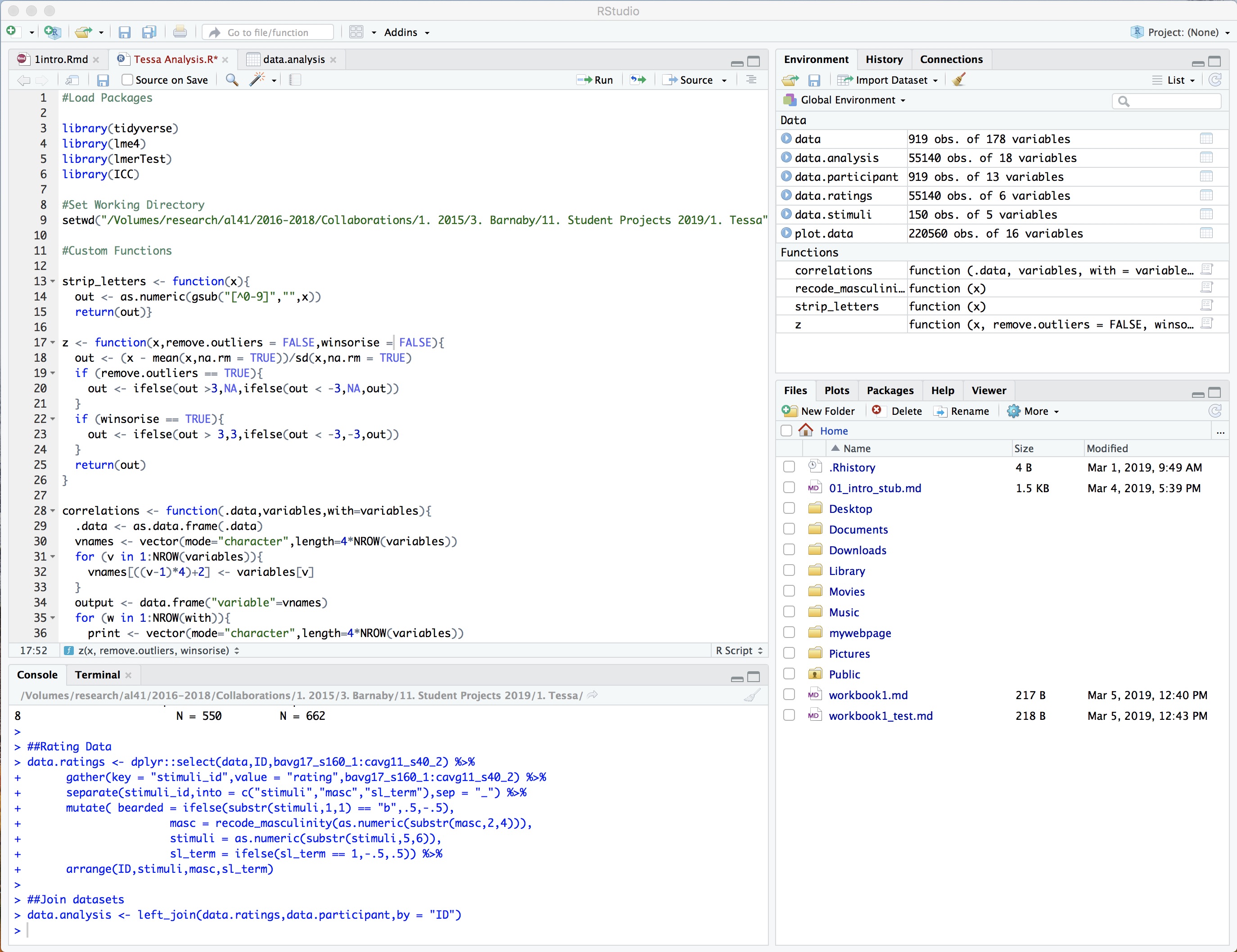
The user interface provides multiple windows in additional to the console that greatly facilitate developing code in R. We will go through each window and their function below:

The bottom left window is the console. This is where you execute code.

The top left window is the script editor. This is where you write and edit your code before sending it to the console. This is what you save when saving your work.

The top right window shows objects in the environment. When coding in R, you will need to save objects to call upon later. Don’t worry too much about this now - we will cover this later in this week’s demonstration content.

Finally, the bottom right window can have various functions, including showing plots, files in the working directory, or show help documentation. We will cover these things in the coming weeks.

Before we start…

We are about to start coding. If you are anxious about coding, know that there are no penalties for making mistakes. R will be good at telling you if something doesn’t work, and when that happens, you will be given unlimited opportunities to try again. A valid coding strategy is just to change something and see what happens.

Also, be prepared to make a lot of typos. Often, these are very simple mistakes that even seasoned programmers make. At times, it may get frustrating, but your ability to spot typos will come with more experience. Common typos include:

Misspelling words/variable names.
Using an underscore (_) instead of a full stop (.) and vice versa.
Capitalising the wrong letters.
Having too many/few brackets.
Having an extra comma somewhere (or missing one).

You will also be exposed to many error messages, and at first they will probably not make a lot of sense to you (copying an error message into Google is an easy way to help find a solution!), but reading through them carefully can give you an indication on where the mistake is. Again, your ability to understand error messages will come with exposure to them.

R as a calculator

We are first going to learn about how to interact with the console (bottom left window). Generally, you will be writing R scripts rather than working directly in the console window. We will be covering more about scripts next week, but a good way to think about it for now is that code entered into the console will happen immediately, while code you draft in a script can be saved for later.

One simple way to learn about the R console is to use it as a calculator. Enter the lines of code below and see if your results match.

1+2

## [1] 3

Remember, R will “read” the command you have typed into the console, evaluated it in the background, and then print the response back to you.

R is not sensitive to spaces, so you can put as many spaces in between your commands as you’d like. This is helpful for long commands, which you can break up over multiple lines.

This…

1 + 2 + 3

## [1] 6

… is the same as this…

1+2+3

## [1] 6

However, you cannot include a space in the middle of the object, so if you are trying to add the numbers “12” and “3” together, the following code will give you an error message.

1 2 + 3

You can also break up commands over multiple lines - this is useful for long commands. When the symbol in the console before the cursor shows a > symbol, it will accept a new command. If it shows a + symbol, R is waiting to receive the end of the previous command. If you want to cancel, press the esc key. For complex functions, it may take R a while to evaluate some code. When R is still thinking, there will be no symbol.

Try running the code below one line at a time.

1 + 2 + 3 +
  4 + 5

## [1] 15

Objects

Often when coding, you will want to store the result of some computation for later use. You can store it as an object. To save something as an object, use the ‘less than’ symbol followed by a dash: <- to assign the name on the right, the value on the left (think of it as an arrow).

The code below saves the evaluation of 1+2 to the object name “x”. Note that when saving an object, it does not print the result back at you.

x <- 1+2

You can then call upon this object later:

## [1] 3

You can also use this object in future commands. The following command takes the object “x” and multiplies it by 2.

x * 2

## [1] 6

Notice that when you save an object, it is added to the list in the top right window of RStudio. This window displays your workspace. Objects in your workspace exist until you overwrite them, clear your workpsace, or until you end your R session. For big projects, it may be helpful to save your workspace, but in general, best practice for reproducible psychological research is to clear your workspace at the end of each session.

Some things to be aware of when naming objects:

Capitalisation matters (e.g., myObject is different to myobject).
You cannot use symbols or spaces, except for underscores _, and periods ..
You can use letters and numbers, but the object name must begin with a letter (b2 is valid, but 2b is not).

Functions

A lot of what you do in R involves calling functions and storing the results. Generally, functions accept objects as arguments, executes a pre-specified set of computations on those objects, then return the result of those computations.

Functions will always follow this general syntax:

function_name(argument1,argument2,argument3,...)

Functions can do different things, depending on the function. Most functions will take an argument (or several arguments), does a specified computation, then return a value. For instance, the sqrt() function below takes one argument (called “x”), which is a number and returns the square root of that number:

sqrt(x = 4)

## [1] 2

Some functions can do quite complicated things. For example, the function rnorm() generates random numbers from the standard normal distribution. This function takes three arguments, where n is the number of randomly generated numbers you want, mean is the mean of the distribution, and sd is the standard deviation. The default mean is 0, and the default standard deviation is 1. So if you want to randomly generate 10 numbers, you can run this code:

rnorm(n = 10,mean = 0,sd = 1)

##  [1]  0.98650688 -0.08376199  0.21938545  0.06008553  2.33667107  1.05697294  0.14839496 -0.65963607
##  [9]  1.17141254  0.26117191

As mentioned above, some arguments have default values, in which case you do not have to specify them. The code below does the same as above, but we do not have to name all the arguments because the defaults for mean and sd are 0 and 1 respectively. However, it is necessary to provide a value for n, as there is no default.

rnorm(n = 10)

##  [1]  0.34143222  0.04837708 -0.77121292  0.28711380 -0.08643160  1.05166925 -0.43576146  2.03475002
##  [9]  0.32137425  0.82929612

If you want to be even more efficient, if you specify your arguments in the order listed for the function, you don’t have to even name them. For example, the code below does the same thing as the two lines above, but since we are specifying the arguments in the specific order, we don’t have to name them.

rnorm(10,0,1)

##  [1] -1.2557397  0.7177088  1.1724181  1.5176900  0.2135408 -0.1283411  0.3036714 -1.0529559 -0.3744430
## [10]  0.2275685

If you have trouble remembering the arguments a particular function takes, you can hover your mouse over the function and a pop up window will give you the function details.

Base R comes with a lot of in-built functions, but one of the great things about R is that there is a large community writing functions and including them in packages for free. Packages are like add-ons that can expand the number of functions you can use in R. We will be covering more about packages next week.

Classes

Up to this point, we have exclusively been dealing with numeric objects, but R can handle various data types (known as classes). There are two that are key to understanding programming in R and content for this module.

Class	Descrption	Example
numeric	Numbers	`1`, `.5`, `-.33`
character	Text String	`"hello world"`, `"something else"`

The general rule is that numeric objects must be a number, and character objects must be contained within quotations (e.g., “this is a character string”).

There are some other class types that are useful to know:

Class	Descrption	Example
factors	A special type of character class where each unique text string represents a separate group (i.e., categories).	`"this is a group"`, `"this is a different group"`
logical (or boolean)	A special type of factor class where the only two valid groups are TRUE and FALSE	`TRUE`, `FALSE`

There are also some other classes (e.g., different types of numeric classes, such as double, and integer), but you don’t have to worry about those for now.

Some functions only work on certain types of classes (e.g., it does not make sense to calculate the square root of a character class!), so it is useful to know what type of class your data is. You can use the class() function to find out.

class(1)

## [1] "numeric"

class("this is a character")

## [1] "character"

class(TRUE)

## [1] "logical"

Vectors

Up to now, we have only been dealing with single values. Often it is necessary to perform a function on several values at once.

Vectors are one of the key structures in R. A vector is like a list of ordered values (called elements). All the elements in a vector must be the same class (e.g., numeric, character). You can create a vector by using the function c(), where each element in your vector is separated by a comma.

The following code makes a numeric vector three elements long.

c(1,2,3)

## [1] 1 2 3

This code makes a character vector five elements long.

c("I","love","statistics","so","much")

## [1] "I"          "love"       "statistics" "so"         "much"

Vectors are useful because it allows R to perform an operation on several values at once. For example, the following code creates an object called “v”, which is a numeric vector. We can then multiply all elements in a vector by three in one line of code. The output of the following code is a three element numeric vector with the answers.

v <- c(1,4,9)

v * 3

## [1]  3 12 27

Some functions can be applied to vectors to perform the operation on all elements at once. For example, the following code gets the square root of each of the numbers in the object v.

sqrt(v)

## [1] 1 2 3

data.frames

In psychological research, one of the main data structures we deal with are data tables (called a data.frame in R). This is what one looks like:

Typically in psychological research, how to read a data table is that each participant is represents a separate row, while different variables that participants can vary on our represented by separate columns (including ID, age, sex, and three other random variables).

So in the data.frame above, participant 1 is a 19-year-old female, while participant 2 is a 22-year-old male. Can you see how to get this information from looking at the table above?

One way of thinking about a data.frame in R is that it is made up of several vectors stacked up next to each other (i.e., each column is a separate vector). If we think of it this way, we can create a data table in R using the data.frame() function, where each argument is a new column, which is a vector with the values. Data.frames can be saved as an object in R.

data <- data.frame(ID = c(1,2,3,4,5),
                   age = c(18,20,21,19,29),
                   sex = c("male","female","female","male","female"),
                   var1 = c(1,4,5,3,7))
data

##   ID age    sex var1
## 1  1  18   male    1
## 2  2  20 female    4
## 3  3  21 female    5
## 4  4  19   male    3
## 5  5  29 female    7

Manually entering data like this is not a particularly efficient way of loading data, and is prone to errors through typos. We will be covering how you can load data saved on your computer into R next week.

There are two ways you can view an entire data.frame in RStudio. The first way, like above, is to type the data.frame object name into the console. However, for big data.frames, this becomes unwieldy. A better way is to use the View() function. Try typing the following code into your console:

View(data)

Looking For Help

We have covered a lot of the basics today, and it’s a lot to take in. While it is good to learn the basic syntax of R coding, note that it is also impossible to commit to memory what every function does in R, and even experienced R programmers will need to look up help or documentation. This can be done in several ways.

Using the help() function. Try running the code below and see what happens. You should see in the bottom right window of RStudio some documentation for the function you’ve asked for help. It will give you a list of arguements the function accepts, and detail on what will be produced. If you scroll to the bottom, you will also see some examples of the function in action.

help(rnorm)

Another way to find help is to Google things. Some useful phrases to Google include: “how to do x in R” or “x function in R”. If you are getting an error message you can’t solve, try copying it into a Google Search. Often, someone on the Internet has previously asked the same question as you, and someone else has already answered it! A good website for this is StackOverflow.

HPSP131 - Workbook 1 - Introduction to R

Objectives

Exercises