Content
These are the packages we will be using in this week’s demonstration.
The lme4 package allows us to conduct the mixed effects
modelling. The lmerTest package is an add-on that
calculates p-values for us. This is the first time we have encountered
both these packages, so make sure to install them before loading
them.
library(tidyverse)
library(lme4)
library(lmerTest)
Linear Mixed Effects Modelling
As covered in lectures, one of the advantages of using Mixed Effects Modelling is when your data violates the assumption of non-independence. A common example is when conducting cross-national research, where responses from different people in the same country may be more similar to each other than responses from people in a different country for reasons not captured in your model. In the following analysis, we will test the influence of age on future discounting behaviour from 13 429 participants from 54 countries.
For a bit of background, future discounting behaviour involves the propensity for people to prefer immediacy over something that is delayed. Future discounting can be measured by asking participants their preference for an immediate reward over a larger, delayed reward (e.g., would you prefer £10 now, or £20 in 60 days?). We can measure a participant’s propensity to future discount by manipulating the difference in rewards, or the length of the delay. Theory would predict that older participants show a greater preference for immediacy compared to younger participants, which we will assess using the data from Lee et al. (2018).
1. Clean data for analysis.
First, we need to calculate a future discounting score for each participant, standardise age, and remove participants with missing data. We also remove participants with unrealistic ages (over 100-years-old or under 6-years-old) and participants from countries where we have less than 10 participants.
data_clean <- fd.data %>%
  drop_na(age,kirby1,kirby2,kirby3,kirby4,kirby5,kirby6,kirby7,kirby8,kirby9) %>%
  mutate(kirby.total = kirby1 + kirby2 + kirby3 + kirby4 + kirby5 + kirby6 + kirby7 + kirby8 + kirby9,
         z.age = c(scale(age))) %>%
  filter(age <= 100) %>%
  filter(age >= 6) %>%
  group_by(resident) %>%
  filter(n() >= 10) %>%
  ungroup()
2. Conduct analysis.
To run a linear mixed effects model, we use the lmer()
function from the lme4 package. We can also load the
lmerTest package, which produces p-values for our mixed
effects models.
Like all analyses conducted in previous demonstrations, we need two things when conducting a mixed effect model: a formula, and a data.frame.
Here is an example of a formula for a mixed effects model:
y ~ x1 + (1 + x1 | group1)
To specify fixed effects, the formula is identical to that of a
normal regression. However, to specify random effects, we need to
introduce some new syntax. In the formula above, random effects are
specified within the brackets, that contains a | symbol.
The variable on the right of the | specifies the grouping
variable. Everything on the left specifies the random effects. A
1 indicates we want a random intercept (i.e., we expect
scores on y to vary depending on group1). Variables on the left hand
side indicate the random slopes we want (i.e., in the example above, we
expect the effect of x1 on y to vary depending on group1).
So in our future discounting analysis, we want the following:
- A fixed effect of participant age - this tells us the effect of age on future discounting and is the relationship we are interested in.
- A random intercept of residence - this accounts for the fact that participants from the same country are more likely to have similar responses to the future discounting measure.
- A random slope of age depending on residence - this accounts for the fact that the effect of age on future discounting may vary according to country of residence.
Altogether, our formula is:
formula <- 'kirby.total ~ z.age + (1 + z.age | resident)'We then feed that into the lmer() function:
model <- lmer(formula,data = data_clean)
summary(model)
## Linear mixed model fit by REML. t-tests use Satterthwaite's method ['lmerModLmerTest']
## Formula: formula
## Data: data_clean
##
## REML criterion at convergence: 53007.9
##
## Scaled residuals:
## Min 1Q Median 3Q Max
## -2.6693 -0.5850 0.0217 0.6116 3.4501
##
## Random effects:
## Groups Name Variance Std.Dev. Corr
## resident (Intercept) 0.09542 0.3089
## z.age 0.15325 0.3915 -1.00
## Residual 3.08354 1.7560
## Number of obs: 13355, groups: resident, 55
##
## Fixed effects:
## Estimate Std. Error df t value Pr(>|t|)
## (Intercept) 3.73685 0.05485 35.21128 68.125 < 2e-16 ***
## z.age 1.31037 0.16282 28.25148 8.048 8.6e-09 ***
## ---
## Signif. codes: 0 '***' 0.001 '**' 0.01 '*' 0.05 '.' 0.1 ' ' 1
##
## Correlation of Fixed Effects:
## (Intr)
## z.age -0.288
## optimizer (nloptwrap) convergence code: 0 (OK)
## boundary (singular) fit: see help('isSingular')In the summary above, there are two tables of interest. In most cases, you will be interested in the ‘fixed effects’ table. This can be interpreted in the same way you would interpret a regression table. So above, we can see that we have a significant, positive effect of age on future discounting; so counter the the hypothesis, older people are more likely to choose the larger future reward. Note that estimates are unstandardised.
The other table is the ‘random effects’ table, which gives you information about variability in your model. So in the example above, scores on future discounting vary by .31 standard deviations depending on residence, the effect of age on future discounting varies by .39 standard deviations depending on residence, while 1.76 standard deviations of future discounting is residual (i.e., not explained by the model).
Sometimes, when running a mixed effect model, you will receive an
error message that says the model failed to converge. This means that R
did not find a single solution, so we cannot be confident in the results
above. If this occurs, the next step is to simplify the random effects
structure. One way to do this is to force the random effects to be
uncorrelated, which can be specified by using two of the |
symbol inside the brackets. For more information on specifying random
effects maximally, read Barr et
al. (2013).
3. Plot the Data
In the plot below, each of the blue lines represents the relationship
between age and future discounting for each country, while the red line
is the overall relationship. This figure is created by adding the
group aesthetic to geom_smooth.
ggplot(data = data_clean,aes(x = age,y = kirby.total)) +
  geom_smooth(aes(group = resident),method = "lm",formula = y ~ x, colour = "blue",se = FALSE,size = .1) +
  geom_smooth(method = "lm",formula = y ~ x, colour = "red")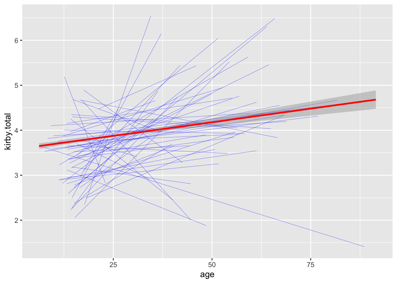
Another Example
In the above example, the level of analysis was at the participant-level. However, since each participant completed 9 inter-temporal choice items, arguably the more appropriate level of analysis is at the item-level (you could expect responses to the same items to be more similar to each other for reasons not measured in the study).
Prepare the data
Up to now, we have required the data to have the structure that one row represents data from one participant. However, this may not be the case when conducting a linear mixed effects model. For a mixed effects model, each row must represent one observation (i.e., Level 1).
For example, let’s say we want to investigate the influences on what participants find attractive in a face, so we conduct a study where each participant rates 9 faces. If we formatted our data so that each participant was on one row, our data would look something like this:
data_short <- data.frame(participant_ID = 1:40,
                         face1 = sample(1:9,40,replace = TRUE),
                         face2 = sample(1:9,40,replace = TRUE),
                         face3 = sample(1:9,40,replace = TRUE),
                         face4 = sample(1:9,40,replace = TRUE),
                         face5 = sample(1:9,40,replace = TRUE),
                         face6 = sample(1:9,40,replace = TRUE),
                         face7 = sample(1:9,40,replace = TRUE),
                         face8 = sample(1:9,40,replace = TRUE),
                         face9 = sample(1:9,40,replace = TRUE))
data_long <- gather(data_short,key = "face",value = "rating",face1:face9) %>%
  arrange(participant_ID,face)
However, to conduct an mixed effects model, we require each row to represent one observation. In this instance, one observation is one rating made by one participant about one face. Therefore, data from one participant would be separated into 9 rows, (one for each rating they gave), and look something like this:
In the examples above, we would call the format of the first
data.frame the “short-form”, while the format for the second is
“long-form”. To convert a data.frame from short-form to long-form and
vice versa, we use the gather() and spread()
functions respectively.
gather()
The gather() function converts data.frames from
short-form to long-form. In order to do this, we first need to specify
two new variable names. First, the ‘key’, which could be considered as
the name for your ‘Trial ID’ (in the example above, this is the
different faces). Second, the ‘value’ variable, which is the name of the
variable you are converting to long-form (in the example above, we have
used ‘rating’). Finally, you need to specify all the variables that you
are converting to long-form. So to covert the data.frame above, the code
looks like this:
data_long <- gather(data_short,key = "face",value = "rating",face1,face2,face3,face4,face5,face6,face7,face8,face9) %>%
  arrange(participant_ID,face)
spread()
If you want to convert back the other way for some reason, you can
use the spread() function. Again, you will need to specify
which column is the ‘key’ and which column is the variable you wish to
convert to short-form. With this information, the spread()
function is smart enough to know what to do:
data_short <- spread(data_long,key = face,value = rating)Actually preparing the data
So, with all that information out of the way, let’s actually convert our future discounting data from short-form to long-form.
data_long <- gather(data_clean,key = "kirby_id",value = "response",kirby1,kirby2,kirby3,kirby4,kirby5,kirby6,kirby7,kirby8,kirby9) %>%
  arrange(user_id,kirby_id)
Run the analysis
As always, now that we have the data.frame prepared for analysis, the only other thing we need is the formula. For the following analysis, we require three random effect groups:
- A random effect of participant.
- A random effect of country.
- A random effect of trial.
We also want to specify random slopes maximally, therefore, we will need a random slope of age for the country group, and the trial group. We do not need one for the participant group, because age does not vary within participants.
Altogether, our formula becomes:
formula <- 'response ~ z.age +
  (1 | user_id) +
  (1 + z.age  || resident) +
  (1 + z.age || kirby_id)'
Note: we use the double || symbol above because a
convergence error when using a single | (and also it just
runs a lot quicker).
We can now run the analysis! Note: given that our dependent variable
is now a dichotomous variable, we need to use the glmer()
function, and specify that the type of analysis is a binomial mixed
effects model using the ‘family’ argument.
model <- glmer(formula,data = data_long,family = "binomial")summary(model)## Generalized linear mixed model fit by maximum likelihood (Laplace Approximation) ['glmerMod']
## Family: binomial ( logit )
## Formula: response ~ z.age + (1 | user_id) + (1 + z.age || resident) + (1 + z.age || kirby_id)
## Data: data_long
##
## AIC BIC logLik -2*log(L) df.resid
## 76864.7 76932.5 -38425.3 76850.7 120188
##
## Scaled residuals:
## Min 1Q Median 3Q Max
## -65.748 -0.250 -0.048 0.203 53.356
##
## Random effects:
## Groups Name Variance Std.Dev.
## user_id (Intercept) 5.617e+00 2.370e+00
## resident (Intercept) 2.865e-01 5.352e-01
## resident.1 z.age 3.076e-10 1.754e-05
## kirby_id (Intercept) 1.385e+01 3.721e+00
## kirby_id.1 z.age 3.336e+00 1.827e+00
## Number of obs: 120195, groups: user_id, 13355; resident, 55; kirby_id, 9
##
## Fixed effects:
## Estimate Std. Error z value Pr(>|z|)
## (Intercept) -1.0518 1.2142 -0.866 0.3864
## z.age 1.1077 0.6512 1.701 0.0889 .
## ---
## Signif. codes: 0 '***' 0.001 '**' 0.01 '*' 0.05 '.' 0.1 ' ' 1
##
## Correlation of Fixed Effects:
## (Intr)
## z.age 0.009
## optimizer (Nelder_Mead) convergence code: 0 (OK)
## boundary (singular) fit: see ?isSingular